Exceedance probability curves
While working on a project proposal to estimate drought risks of some countries in the coming years, I learned something about risk analysis: It’s rather simple! But, you need to be cautious if you want to use this information for guessing what might happen in the future. In the context of anthropogenic climate change that usually means that you can’t rely on exceedance probabilities from observed (and hence past) data. Because the underlying climate is changing. And even if that’s not the case, your record may be over- or underestimating the occurrences of specific events, just by pure chance.
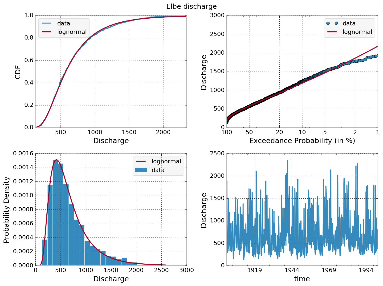
However, let me show you how to quickly derive exceedance probabilities from some river discharge data.
From the monthly discharge data, we estimate the cumulative distribution function (CDF) by assigning each sorted monthly value a number starting from 0 for the lowest up to 1 for the highest monthly discharge value. The exceedance probability is simply 1 - CDF. Plotting the exceedance probability against the sorted monthly data, et voilà, your exceedance probability curve.
Here’s the link to the CSV file elbe.csv and the Python code to process the data.
import matplotlib.pyplot as plt
import pandas as pd
import numpy as np
from scipy import stats
import sys
import matplotlib
from matplotlib.ticker import ScalarFormatter, FormatStrFormatter, FixedLocator

matplotlib.style.use('bmh')

fnm  = 'elbe.csv'
df = pd.read_csv(fnm,index_col=0,infer_datetime_format=True,parse_dates=True)
raw = df['Elbe']
ser = raw.sort_values()

X = np.linspace(0.,max(ser.values)*1.1,100.)
s, loc, scale = stats.lognorm.fit(ser.values)

cum_dist = np.linspace(0.,1.,len(ser))
ser_cdf = pd.Series(cum_dist, index=ser)
ep = 1. - ser_cdf

fig = plt.figure(figsize=(11,8))

ax1 = plt.subplot(221)
ser_cdf.plot(ax=ax1,drawstyle='steps',label='data')
ax1.plot(X,stats.lognorm.cdf(X, s, loc, scale),label='lognormal')
ax1.set_xlabel('Discharge')
ax1.set_ylabel('CDF')
ax1.legend(loc=0,framealpha=0.5,fontsize=12)

ax2 = plt.subplot(223)
ax2.hist(ser.values, bins=21, normed=True, label='data')
ax2.plot(X,stats.lognorm.pdf(X, s, loc, scale),label='lognormal')
ax2.set_ylabel('Probability Density')
ax2.set_xlabel('Discharge')
ax2.legend(loc=0,framealpha=0.5,fontsize=12)

A = np.vstack([ep.values, np.ones(len(ep.values))]).T
[m, c], resid = np.linalg.lstsq(A, ser.values)[:2]
print(m, c)
r2 = 1 - resid / (len(ser.values) * np.var(ser.values))
print(r2)

ax3 = plt.subplot(222)
ax3.semilogx(100.*ep,ser.values,ls='',marker='o',label='data')
ax3.plot(100.*(1.-stats.lognorm.cdf(X, s, loc, scale)),X,label='lognormal')
minorLocator = FixedLocator([1,2,5,10,20,50,100])
ax3.xaxis.set_major_locator(minorLocator)
ax3.xaxis.set_major_formatter(ScalarFormatter())
ax3.xaxis.set_major_formatter(FormatStrFormatter("%d"))
ax3.set_xlim(1,100)
ax3.set_xlabel('Exceedance Probability (%)')
ax3.set_ylabel('Discharge')
ax3.invert_xaxis()
ax3.legend(loc=0,framealpha=0.5,fontsize=12)

ax4 = plt.subplot(224)
raw.plot(ax=ax4)
ax4.set_xlabel('time')
ax4.set_ylabel('Discharge')

plt.suptitle('Elbe discharge',y=1.01,fontsize=14)

plt.tight_layout()
plt.show()

fig.savefig('exceedance_curve_elbe.png',transparent=True,dpi=150,bbox_inches='tight')