How to calculate the heat flux within a snowpack
It sounds simple but requires at least some basic knowledge of partial differential equations. You also need to know about discretisation so that you can solve the equation
\[c_p \rho_w\frac{\partial T}{\partial t} = K \frac{\partial^2 T}{\partial x^2}\]on your computer. Most commonly used are finite difference schemes, for example, explicit (forward time stepping), implicit (backward time stepping), or the Crank-Nicolson (both, forward and backward time stepping) schemes.
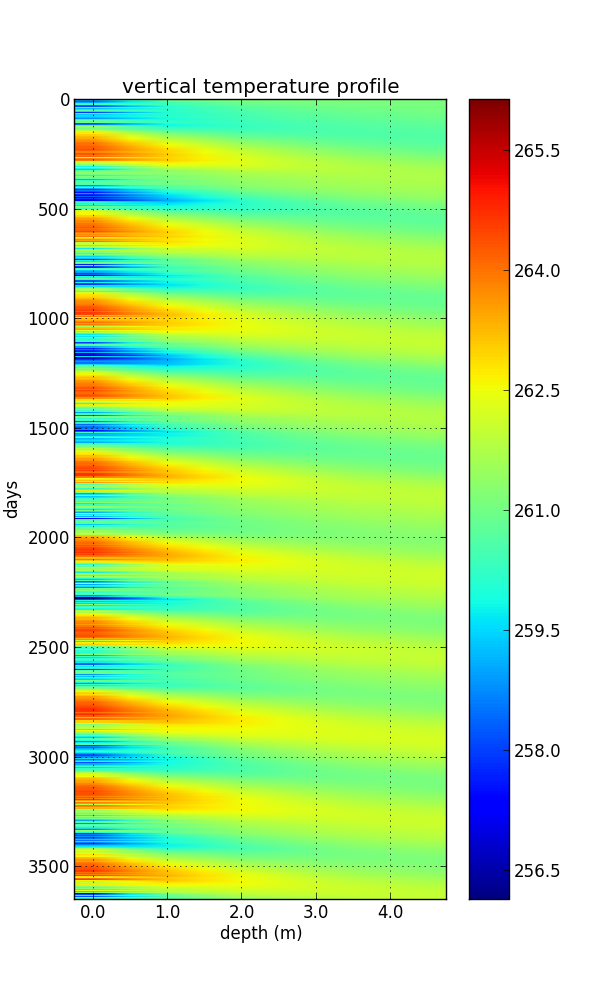
Here you see an example of a vertical temperature profile of a snowpack of 5m thickness. On top (left, 0m) the model is forced with 10 years of surface temperature at location of the JAR automatic weather station as modelled by MAR. You can see the alternating summer and winter heat and cold waves entering the snowpack. The annual cycle is the strongest because a slower surface signal (i.e., longer time scales) lead to a larger penetration depth ($l$)
\[l = \sqrt{2\,\frac{K}{c_p \rho_w} \Delta t}\]Because of the (almost) periodic forcing the signal at depth is phase shifted and decays exponentially.